Combining categories of ordinal data: what you lose by dichotomizing

Ordinal scales are common in surveys for master’s and doctoral theses. Take an example: respondents rate their health as very good, good, fair, poor or very poor. When it is time for analysis, it is tempting to reduce the answers to two groups, favourable and unfavourable health.

This sounds reasonable, but such a simplification can change the conclusion you draw from the data. In this guide I explain exactly what you lose by merging categories and what you can do instead.

What dichotomization is and why it is tempting

Dichotomization means turning a variable with several categories, or a continuous variable, into a variable with only two values. The result is easy to describe with a single percentage, and the analysis comes down to familiar tools: the chi-square test, the odds ratio or binary logistic regression.

That simplicity is exactly why dichotomization is used even when there is no good reason for it. The methodological literature, for example the review by MacCallum and colleagues in Psychological Methods, has long warned that the price of this simplification is higher than it first appears.

What you lose when you merge categories

Differences within a group. Once “very good” and “good” are merged, they become the same answer. If a respondent’s health declines from very good to good, the dichotomous variable does not show that change. You can think of an ordinal scale as a continuous sense of health cut into five bands; merging bands makes that cut even coarser.

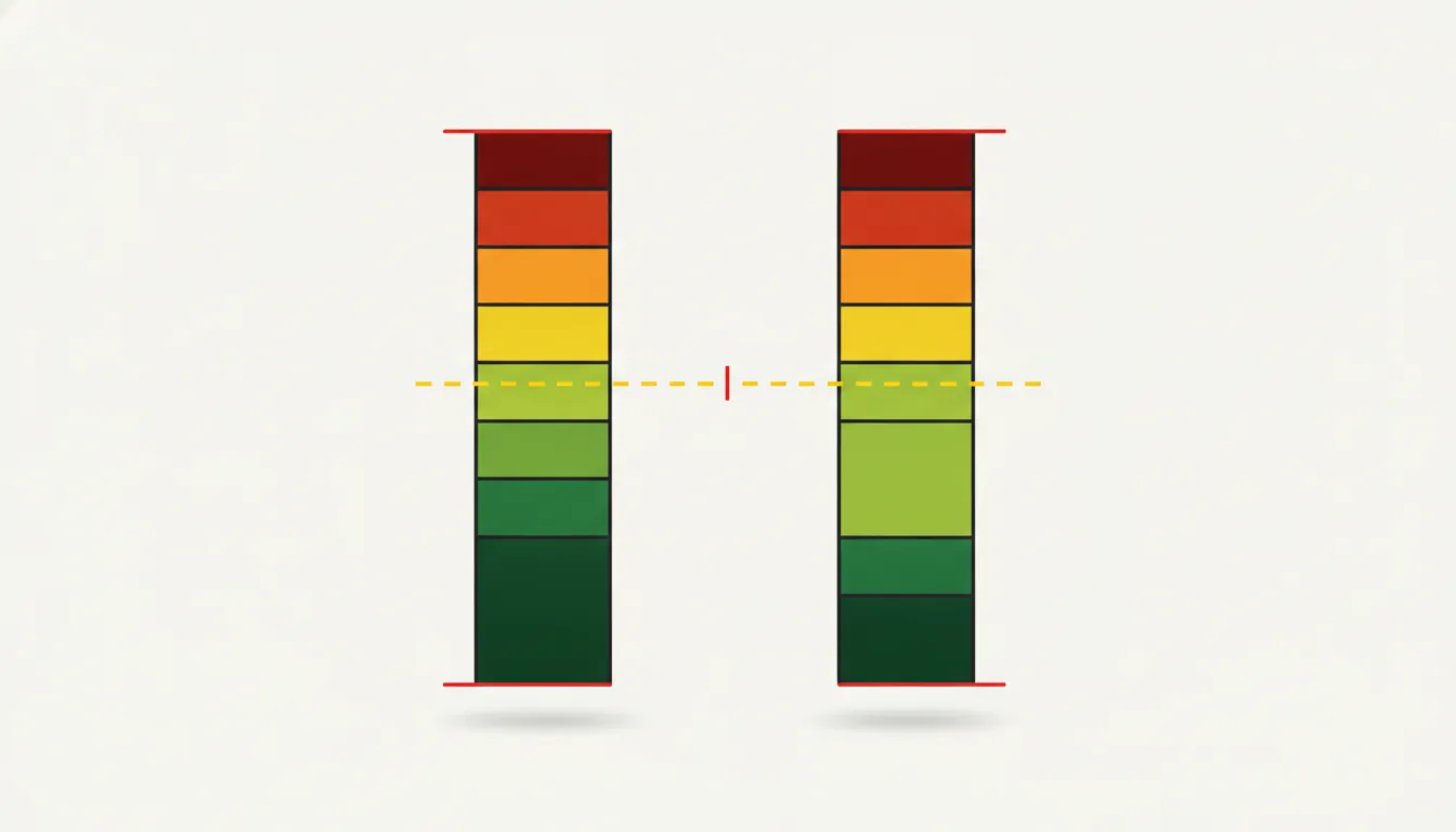The same share of favourable answers, but a different distribution within the group. · Illustration: AI-generated

Differences between groups. Two groups can have the same share of favourable answers and a completely different distribution. In one, most choose “very good”; in the other, “good”. A dichotomous analysis will tell you they are the same.

Statistical power. Less information means less precise estimates. The paper mentioned above shows that dichotomization generally weakens the observed association between variables, so you need a larger sample to detect the same difference and you are more likely to miss an effect that really exists.

Apparent jumps. A respondent who moves from “fair” to “good” crosses the cut-off and looks like a big change, while a larger shift within the same group remains invisible.

Spurious findings. Losing information does not always just make conclusions more cautious. When several predictors are dichotomized at once, effects or interactions can appear that do not exist in the original data.

Where to draw the line?

With a scale that has an odd number of responses, the problem is the middle category. Does “fair” belong to favourable or unfavourable health? The answer can change the result, and sometimes even the direction of the conclusion.

A further difficulty is that the distances between categories need not be equal. The gap between “unlikely” and “somewhat likely” may be smaller than the one between “somewhat” and “very likely”, so a “natural midpoint” of the scale often does not exist at all.

It is especially risky to choose the cut-off after looking at the data. You can then easily, and unconsciously, pick the split that gives a statistically significant result, which increases the chance of a false positive. Reviewers and supervisors are keen to ask about this.

Better alternatives

• Show the full distribution: with a frequency table or a stacked bar chart by group.
• Use tests for ordinal data: the Mann-Whitney U test for two groups, the Kruskal-Wallis test for more groups, a trend test for tables with ordered categories, or Spearman’s correlation.
• For modelling, use ordinal logistic regression (the proportional odds model) and check its proportional odds assumption.

Ordinary linear regression is not a good substitute because it treats categories as equally spaced numbers, and multinomial logistic regression ignores the ordering and thereby discards part of the information. The ordinal model treats the categories as cuts of a latent continuous variable and estimates the thresholds between them. The resulting proportional odds ratio is interpreted much like one from binary logistic regression, but it applies to every “higher versus lower” split. In other words, the model uses all possible dichotomizations at once instead of you choosing one. In R it is fitted with the polr function from the MASS package, and the ordered probit gives very similar results, differing mainly in how the coefficients are interpreted.

Be careful when checking the assumption: formal tests tend to reject it even when it actually holds. A graphical approach recommended by Harrell, comparing predicted logits for each outcome cut-off, is therefore useful too. If the assumption clearly fails, consider a model that allows different coefficients for different cut-offs.

These approaches keep the order of the categories and do not require an arbitrary cut-off.

If you must merge categories anyway

There are legitimate reasons: a clinically or practically important threshold, comparability with earlier studies, or too few responses in the extreme categories. In that case:

1. Set the cut-off in advance, in the analysis plan.
2. Justify the choice in the methods section.
3. Run a sensitivity analysis with a different cut-off and check whether the conclusion changes.
4. Alongside the dichotomous result, show the full distribution of responses and, if possible, the result of an ordinal model.

In short

• Merging categories hides differences within and between groups.
• It reduces statistical power and can create apparent jumps, or even spurious effects.
• The choice of cut-off affects the result, especially with a middle category and unequal spacing.
• Ordinal data are best analysed with ordinal methods, with a sensible check of proportional odds.
• If you dichotomize, set the cut-off in advance, justify it and test it with a sensitivity analysis.

Cover: AI-generated